2D Inversion Sampling with Images | Christopher M. Pierce

Inversion sampling (also mentioned here) is interesting because as long as the target distribution is integrable and that integral is invertible, you can draw samples from it efficiently. These operations can also happen numerically allowing for sampling from distributions that are defined numerically.

In 2D, things are a little more convoluted, but we can still handle each coordinate one at a time. We draw one variable ($y$ here) from its marginal distribution, then for each element in the sample, draw the other variable ($x$) from its conditional distribution given the corresponding value of $y$. That is, if we draw two samples from uniformly distributed random variables on [0, 1], the transformed samples are the following.

\[y_s = \text{CDF}_{y}^{-1}(v),\] \[x_s = \text{CDF}^{-1}_{y=y_s}(u),\]

Where $\text{CDF}y$ means the CDF of y’s marginal distribution ($\rho(y) = \int \rho(x, y) \mathrm{d}x$) and $\text{CDF}{y=y^\prime}$ is the CDF of the conditional distribution of $x$ given the sampled value of $y$, $\rho(x

y) = \rho(x, y)/\rho(y)$.

Since this method is easy to evaluate numerically, we can do fun things like consider the pixel intensities inside of an image as defining a probability distribution and drawing samples from it. The following python code will do this.

def sample_2d_image(rho, n_samp):
    # Integrate to get cumulative distributions
    rho_x = np.cumsum(rho, axis=0)
    rho_xy = np.cumsum(rho_x[-1, :])

    # Generate random variables on [0, 1]x[0, 1]
    u, v = np.random.random((2, n_samp))

    # Transform to get the column
    n = np.interp(v, rho_xy / rho_xy[-1], np.arange(0, rho_xy.shape[0]))

    # For each variable, get the index to the column we are in
    m = np.zeros_like(n)
    samps_n_idx = np.searchsorted(np.arange(0, rho_xy.shape[0]), n)

    # For each of the columns, select all samples in it and invert CDF to find row coordinate
    for n_idx in range(rho.shape[1]):
        filt = samps_n_idx == n_idx
        m[filt] = np.interp(
            u[filt],
            rho_x[:, n_idx] / (1e-19 + rho_x[-1, n_idx]),
            np.arange(0, rho_x.shape[0]),
        )
    return m, n

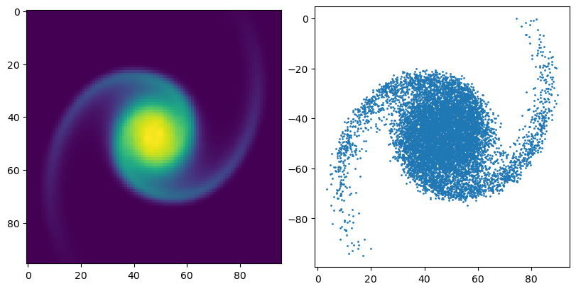
As an experiment, we can take some 2D histograms of electron beams and turn them back into samples. Overlaying the density back with itself, we can visually see that things line up. Note, I am flipping the sign of $m$ for plotting to deal with mixed conventions for images and scatter plots.

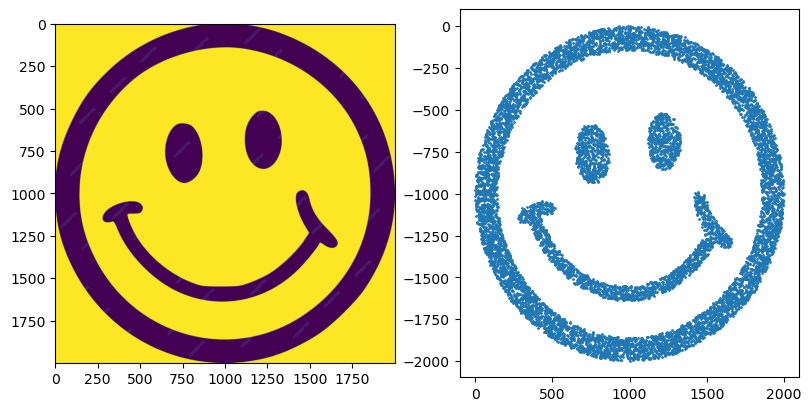
Inversion sampling from beam distribution.

We can also sample from more interesting distributions.

Fun example of inversion sampling.

Note: this is the method used in Distgen and looking over the source code helped me with the image sampling problem. Go check out the repo and toss a Github star their way.