Learning Implicit Particle Beam Representations

In accelerator physics, a key representation of particle beams is their density in phase space. In our 3D world, this takes the form of the function $\rho(x, p_x, y, p_y, z, p_z)$, but for the purposes of a machine learning experiment we may consider data from a simple one dimensional system and the corresponding beam $\rho(x, p_x)$. Here, data on the beam takes the form of images encoding density within some bounding box around the beam. These images could be learned directly, but it is interesting to instead learn the function $\rho(x, p_x, \vec{\Theta})$ directly for some system parameters $\vec{\Theta}$. This is called an implicit neural representation and has some writing on it already.

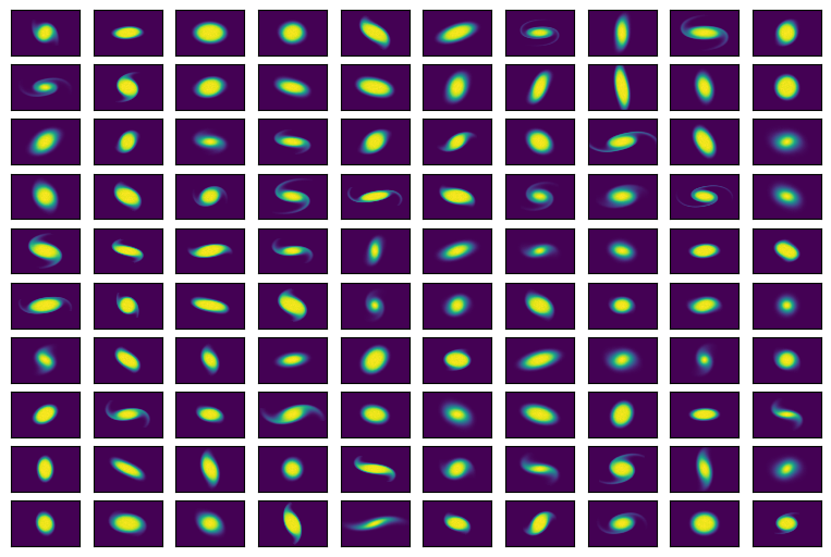
Using a particle tracking code, I have already generated a dataset of 1D electron beams in a uniform focusing channel with space charge for a variety of system and initial parameters. The initial beam was supergaussian and I varied the following (with some descriptions for those not used to accelerator physics jargon).

• Initial Twiss beta (the initial ratio of the beam’s size in $x$ and $p_x$)
• Initial Twiss alpha (the initial correlation between $x$ and $p_x$)
• Initial emittance (beam’s initial area in phase space)
• Supergaussian “n” of initial distribution (how “sharp” is the initial distribution)
• Beam perveance (bunch charge, controls amount of space charge forces… ie the repulsion of the beam away from itself.)
• Channel focusing strength (how strongly does the external focusing element affect the beam) Here are some example images.

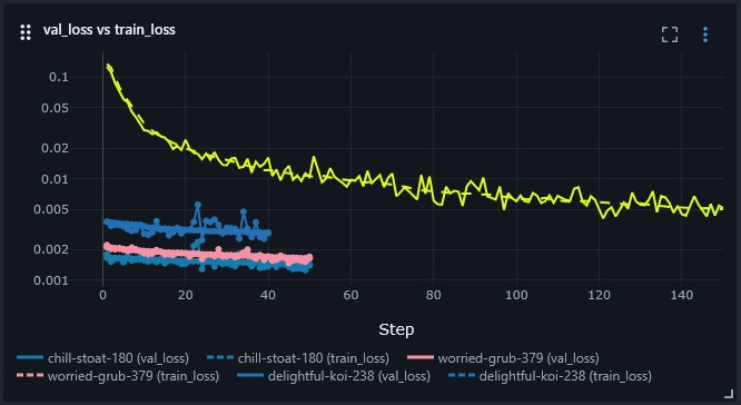
Using an MLP with $\exp(x)$ tacked onto the end, I was able to successfully learn the implicit representation of the data. This simple model makes sense as all of the densities should look a bit like supergaussians $A\cdot\exp\left[-\left(x^2 + p_x^2\right)^n\right]$ with various simple nonlinear mappings of $x$ and $p_x$ applied. The MLP should be ok at learning the stuff inside $\exp(\cdots)$. This ended up taking more compute than I was expecting for the system, but I suppose the number of parameters ended up being ambitious and the number of training samples is large considering each pixel in the images counts. Training went well with the learning rate getting dropped after successive rounds. I found that a fairly large learning rate was needed to get the model to start to look “beam-like” at all and then a lower learning rate is needed to begin representing details in the image.

As an experiment in deploying models, I am embedding a viewer directly into this post. Try hitting “play” in the window below. The plots being shown are not video, these are the output of a neural network with inference being done directly in your browser. Go ahead and change the knobs and explore the dataset.

This simple model has some “stripe” artifacts in it which I would like to work out. I believe regularization will help.