The 2D supergaussian distribution is useful for describing electron beams generated from lasers that can vary from Gaussian to flat-top in shape. To simulate these beams in a particle tracking code, samples I need a method to generate samples from this distribution numerically. In this note, I derive formulas to do just that using inversion sampling.

Inversion Sampling

A neat, efficient way of generating samples from an arbitrary distribution is inversion sampling. First, we generate samples over $[0, 1]$ from the uniform distribution ($\rho_u$). Then, we transform them by the inverse of the cummulative density function (CDF) of the desired distribution ($\rho_d$). Let’s calculate the resulting density of the transformed samples knowing that densities transform with the determinant of the Jacobian out front.

We can simplfy this. First off, $\rho_u(\text{CDF}^{-1}(x^\prime))$ is one everywhere since we began with the uniform distribution which is $\rho_u(x) = 1$ over $[0, 1]$ and the CDF maps from the domain of our desired distribution onto $[0, 1]$. The second simplification is that the CDF is just the integral of the PDF of our desired distribution. This means $\left[ \frac{d [\text{CDF}]}{d x^\prime}\right]_{x^\prime} = \rho_d(x’)$. Therefore, the transformed density is,

We can therefore create samples from the desired distribution by drawing samples from the uniform distribution over $[0, 1]$ and applying the transformation $\text{CDF}^{-1}(x)$. Note that unlike rejection sampling, every sample we begin with ends up in the final samples. However, we must be able to evaluate $\text{CDF}^{-1}(x)$ efficiently.

Inverse CDF of Supergaussian

There are multiple ways of defining the supergaussian distribution, but for this note I will use the convention,

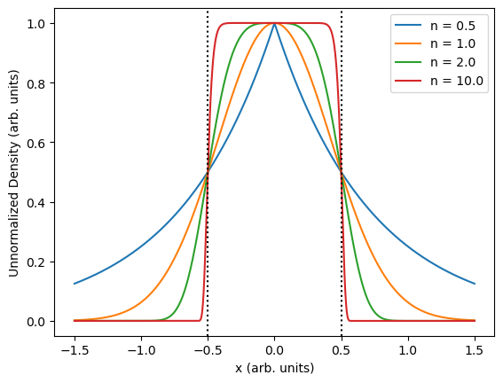
This variant is symmetric in $x$ and $y$ and has a full width at half maximum of one. I don’t include variance/covariance as parameters here as they can be trivially applied to the resulting samples through a linear transformation after generation. A figure showing the density for different values of $n$ with $y=0$ is shown at the top of this note.

Note that a transformation to polar coordinates naturally expresses the rotational symmetry of the density. Doing this and being careful to multiply by the determinant of the Jacobian to preserve the interpretation of $\rho$ as a probability density function (PDF) gives,

Since the PDF is separable, we can draw samples for $\theta$ (uniformly distributed) and $r$ (distributed accoring to the above equation) separately, then transform into cartesian coordinates. To use inversion sampling for $r$, we must calculate the inverse of its CDF

Integrating the previous equation and then setting $A$ so that $\lim\limits_{r\to\infty} \text{CDF}(r) = 1$ gives,

where $\Gamma(x)$ and $\Gamma(a, x)$ are the complete and upper incomplete gamma functions respectively.

This CDF isn’t invertible in terms of common functions. However, many popular numerical libraries (such as scipy and boost) contain methods to efficiently calculate the inverse of the incomplete Gamma functions. Solving the problem in terms of the inverse regularized gamma function (I use the convention of gamma_q_inv from boost), the inverse CDF is,

Generating Samples in Python

To recap, I have calculated the inverse CDF of the radial part of the supergaussian distribution in polar coordinates. To generate a sample, we first generate two uniformly distributed random numbers, the first is transformed by the inverse of the CDF we found to get $r$. The second is rescaled to $[0, 2\pi]$ to give us $\theta$. The coordinates are the then transformed to cartesian coordinates.

The following python code implements this.

from scipy.special import gammainccinv
import numpy as np

def sample_supergaussian(n, n_samp):
    # Start with uniform random samples
    u = np.random.random(n_samp)
    v = np.random.random(n_samp)

    # Transform by inverse CDF of dist in polar coordinates
    theta = 2*np.pi*u
    r = 0.5*np.power(gammainccinv(1/n, (1-v))/np.log(2), 1/2/n)

    # Transform to Cartesian coordinates
    x = r*np.cos(theta)
    y = r*np.sin(theta)

    return x, y

This code generates the following samples. Remember that in my convention, $n=1$ is a Gaussian distribution, $n\to\inf$ is flat-top.

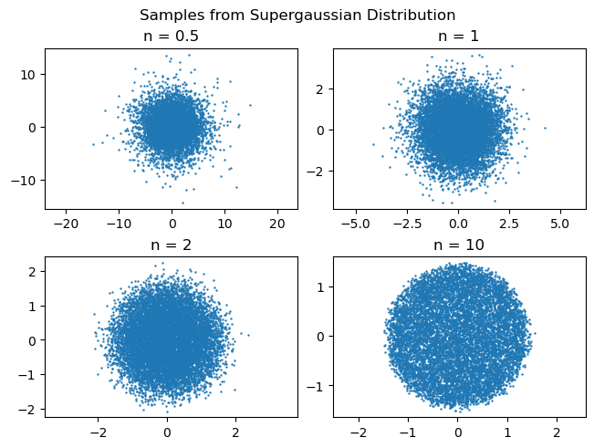
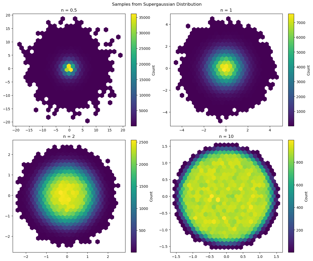
The samples behave qualitatively as expected. Plotting the densities using a histogram also helps to confirm that the method works.

Miscellaneous Notes

• The PDF is also separable in Cartesian coordinates, but will give a similar CDF in terms of gamma functions. Generating the samples in polar coordinates reduces the number of calls to the inverse gamma function by a factor of two (only one for $r$ instead of one each for $x$ and $y$) which is desirable because it is the most computationally expensive part of the process.